EMVS: The EM Approach to Bayesian Variable Selection

Caleb Jin / 2017-12-15

Introduction

The EMVS (Rockova and George 2014) method is anchored by EM algorithm and original stochastic search variable selection (SSVS). It is a deterministic alternative to MCMC stochastic search and ideally suited for high-dimensional $p > n$ settings. Furthermore, EMVS is able to effectively identify the sparse high-probability model and find candidate models within a fraction of the time needed by SSVS. This algorithm makes it possible to carry out dynamic posterior exploration for the identification of posterior modes.

The outline of this course project is as follows. In section 2, we build original SSVS method, including its prior and posterior distribution for each parameter. In section 3, I derive the author’s new idea EMVS method in very details that the author omits. In section 4, I perform several simulation case studies from this paper and me, then compare the results of SSVS and EMVS.

Stochastic Search Variable Selection (SSVS)

Model Settings

Consider a multiple linear regression model as follows:

\begin{array}{rcl} (1) & y = X β + ϵ, \end{array}

where

y = (y_{1}, \dots, y_{n})^{⊤}

is the

n

-dimensional response vector,

X = [x_{1}, \dots, x_{n}]^{⊤}

is the

n \times p

design matrix,

β = (β_{1}, β_{2}, \dots, β_{p})^{'}

σ^{2}

is a scalar, and

ϵ \sim N_{n} (0, σ^{2} I_{n})

. Both

σ^{2}

and

β

are considerd bo te unknown. We assume that

p > n

. From (1), the likelihood function is given as

\begin{array}{rcl} y | β, σ^{2} \sim N (X β, σ^{2} I_{n}) . \end{array}

The cornerstone of $SSVS$ is the “spike and slab” Gaussian mixture prior on $β$ , $\begin{array}{rcl} β_{j} | σ^{2}, γ_{j} \overset{i n d}{\sim} (1 - γ_{j}) N (0, σ^{2} ν_{0}) + γ_{j} N (0, σ^{2} ν_{1}), \end{array}$ where $\begin{array}{rcl} (2) & γ_{j} = {\begin{array}{lcr} 1 & β_{j} \neq 0 \\ 0 & β_{j} = 0, \end{array} \end{array}$ $j = 1, 2, \dots, p$ . $0 \leq ν_{0} < ν_{1}$ .

Hence, $β | σ^{2}, γ \sim N_{p} (0, D_{σ^{2}, γ})$ , where $D_{σ^{2}, γ} = σ^{2} d i a g (ν_{z_{1}}, ν_{z_{1}}, \dots, ν_{z_{p}})$ .

For the prior on the $σ^{2}$ , I follow the (George and McCulloch 1997) and use inverse gamma prior but different notation, $\begin{array}{rcl} σ^{2} \sim I G (\frac{a}{2}, \frac{b}{2}), \end{array}$ where we will use $a = 1$ and $b = 1$ , and $σ^{2}$ is also independent of $γ$ .

I follow the (George and McCulloch 1997) and use Bernoulli prior form but different notation, $\begin{array}{rcl} γ_{j} | θ \overset{i i d}{\sim} B e r (θ), θ \in [0, 1] . \end{array}$ Hence, $\begin{array}{rcl} (3) & γ \propto θ^{\sum_{j = 1}^{p} γ_{j}} (1 - θ)^{p - \sum_{j = 1}^{p} γ_{j}} \end{array}$ We assume $\begin{array}{rcl} θ \sim B (c_{1}, c_{2}), \end{array}$ where we will use $c_{1} = c_{2} = 1$ , which leads to the uniform distribution.

It is easy to show that the full conditionals are as follows:

1. $β_{j} | β_{- j}, σ^{2}, γ, ν_{0}, y \sim N ({\tilde{β}}_{j}, \frac{σ^{2}}{μ_{j}}) .$ where $μ_{j} = x_{j}^{⊤} x_{j} + \frac{1}{ν_{γ_{j}}}$ and ${\tilde{β}}_{j} = μ_{j}^{- 1} x_{j}^{⊤} (y - X_{- j} β_{- j})$ .
1. $\begin{array}{rcl} γ_{j} | γ_{- j}, β, σ^{2}, y \sim B e r (\frac{ν_{1}^{- \frac{1}{2}} \exp (- \frac{1}{2 σ^{2} ν_{1}} β_{j}^{2}) θ}{ν_{0}^{- \frac{1}{2}} \exp (- \frac{1}{2 σ^{2} ν_{0}} β_{j}^{2}) (1 - θ) + ν_{1}^{- \frac{1}{2}} \exp (- \frac{1}{2 σ^{2} ν_{1}} β_{j}^{2}) θ}) . \end{array}$
1. $σ^{2} | β, γ, y \sim I G (a^{*}, b^{*}) .$ where $a^{*} = \frac{1}{2} (n + p + a)$ and $b^{*} = \frac{1}{2} (‖ y - X β ‖^{2} + \sum_{j = 1}^{p} \frac{β_{j}^{2}}{ν_{γ_{j}}} + b) .$
1. For $θ | γ$ , we have

$\begin{aligned} π (θ | γ) & \propto π (γ | θ) π (θ) \\ \propto [\prod_{j = 1}^{p} θ^{γ_{j}} (1 - θ)^{1 - γ_{j}}] θ^{c_{1} - 1} (1 - θ)^{c_{2} - 1} \\ \propto θ^{\sum_{j = 1}^{p} γ_{j} + c_{1} - 1} (1 - θ)^{p - \sum_{j = 1}^{p} γ_{j} + c_{2} - 1}, \end{aligned}$ where we will use $c_{1} = c_{2} = 1$ , which leads to the uniform distribution. We therefore have $\begin{array}{rcl} θ | γ \sim B (\sum_{j = 1}^{p} γ_{j} + c_{1}, p - \sum_{j = 1}^{p} γ_{j} + c_{2}) . \end{array}$

EMVS

Genared toward finding posterior modes of the parameter posterior $π (β, σ^{2}, θ | y)$ rather than simulating from the entire model posterior $π (γ | y)$ , the EM algorithm derived here offers potentially enormous computational savings over stochastic search alternatives, especially in problems with a large number p of potential predictors.

$EMVS$ consists of two steps: E-Step, conditional expectation given the observed data and current parameter estimates, and M-Step, entails the maximization of the expected complete data log posterior with respect to $(β, σ^{2}, θ)$ .

Define $ϕ = (β, σ^{2}, θ)$ . EM algorithm maximizes $π (ϕ | y)$ by iteratively maximizing the objective function $\begin{array}{rcl} Q (ϕ | ϕ^{(t - 1)}, y) = E_{γ | \cdot} [\log π (ϕ, γ | y)], \end{array}$ where $E_{γ | \cdot}$ denotes $E_{γ | ϕ^{(t - 1)}, y}$ .

According to the class note, it can be written as $\begin{array}{rcl} (4) & Q^{⋆} (ϕ | ϕ^{(t - 1)}, y) = E_{γ | \cdot} [\log π (ϕ | γ, y)] \end{array}$ At the $(t - 1)$ th iteration, given $ϕ^{(t - 1)}$ , an E-step is first applied, which computes the expectation of the right side of (4) to obtain $Q$ . This is followed by M-step, which maximizes $Q$ over $(β, σ^{2}, θ)$ to obtain $(β^{(t)}, σ^{2 (t)}, θ^{(t)})$ .

$\begin{array}{rcl} Q^{⋆} (β, σ^{2}, θ | β^{(t)}, σ^{2 (t)}, θ^{(t)}, y) \\ = & Q^{⋆} (β, σ^{2}, θ | ϕ^{(t - 1)}, y) \\ = & C + Q_{1} (β, σ^{2} | ϕ^{(t - 1)}, y) + Q_{2} (θ | ϕ^{(t - 1)}, y) \\ = & C + E_{γ | \cdot} [\log π (β, σ^{2} | ϕ^{(t - 1)}, y)] + E_{γ | \cdot} [\log π (θ | ϕ^{(t - 1)}, y)] \end{array}$

1. $Q_{1} (β, σ^{2} | ϕ^{(t - 1)}, y)$ $\begin{array}{rcl} π (β, σ^{2} | ϕ^{(t - 1)}, y) \\ \propto & π (y | β, σ^{2}) π (β | σ^{2}, γ) π (σ^{2}) \\ \propto & (σ^{2})^{- \frac{n}{2}} \exp (- \frac{1}{2 σ^{2}} | | y - x β | |^{2}) (σ^{2})^{- \frac{p}{2}} \prod_{j = 1}^{p} ν_{γ_{j}} \exp (- \frac{1}{2 σ^{2} ν_{γ_{j}}} β_{j}^{2}) \\ \times (σ^{2})^{- \frac{a}{2} - 1} \exp (- \frac{b}{2 σ^{2}}) \\ \propto & (σ^{2})^{- \frac{n + p + a + 2}{2}} \exp [- \frac{1}{2 σ^{2}} (| | y - x β | |^{2} + \sum_{j = 1}^{p} β_{j}^{2} \frac{1}{ν_{γ_{j}}} + b)] \end{array}$

$\begin{array}{rcl} Q_{1} (β, σ^{2} | ϕ^{(t - 1)}, y) \\ = & E_{γ | \cdot} [\log (π (β, σ^{2} | ϕ^{(t - 1)}, y))] \\ = & - \frac{1}{2} (n + p + a + 2) \log (σ^{2}) - \frac{1}{2 σ^{2}} (| | y - x β | |^{2} + b) - \frac{1}{2 σ^{2}} \sum_{j = 1}^{p} β_{j}^{2} E_{γ | \cdot} [\frac{1}{ν_{γ_{j}}}] \end{array}$

1. $Q_{2} (θ | ϕ^{(t - 1)}, y)$ $\begin{array}{rcl} π (θ | γ, y) \\ \propto & π (γ | θ) p (θ) \\ \propto & θ^{\sum_{j = 1}^{p} γ_{j} + c_{1} - 1} (1 - θ)^{p - \sum_{j = 1}^{p} γ_{j} + c_{2} - 1} \end{array}$

$\begin{array}{rcl} \log (π (θ | γ, y)) \\ = & C + (\sum_{j = 1}^{p} γ_{j} + c_{1} - 1) \log θ + (p - \sum_{j = 1}^{p} γ_{j} + c_{2} - 1) \log (1 - θ) \\ = & C + \log \frac{θ}{1 - θ} \sum_{j = 1}^{p} γ_{j} + (c_{1} - 1) \log θ + (p + c_{2} - 1) \log (1 - θ) \end{array}$

$\begin{array}{rcl} Q_{2} (θ | ϕ^{(t - 1)}, y) \\ = & \log \frac{θ}{1 - θ} \sum_{j = 1}^{p} E_{γ | \cdot} [γ_{j}] + (c_{1} - 1) \log θ + (p + c_{2} - 1) \log (1 - θ) \end{array}$

The E-Step

The E-step proceeds by computing the conditional expectations $E_{γ | \cdot} [\frac{1}{ν_{γ_{j}}}]$ and $E_{γ | \cdot} [γ_{j}]$ for $Q_{1}$ and $Q_{2}$ , respectively.

1. For $E_{γ | \cdot} [γ_{j}]$ ,

$\begin{array}{rcl} π (γ_{j} | θ, β_{j}, σ^{2}, y) \\ \propto & π (β_{j} | γ_{j}, σ^{2}) p (γ_{j} | θ) \\ \propto & ν_{γ_{j}}^{- \frac{1}{2}} \exp (- \frac{1}{2 σ^{2} ν_{γ_{j}}} β_{j}^{2}) θ^{γ_{j}} (1 - θ)^{1 - γ_{j}} \end{array}$

Hence, $π (γ_{j} = 1 | θ, β_{j}, σ^{2}, y) = C ν_{1}^{- \frac{1}{2}} \exp (- \frac{1}{2 σ^{2} ν_{1}} β_{j}^{2}) θ \equiv a_{i}$ ,

$π (γ_{j} = 0 | θ, β_{j}, σ^{2}, y) = C ν_{0}^{- \frac{1}{2}} \exp (- \frac{1}{2 σ^{2} ν_{0}} β_{j}^{2}) (1 - θ) \equiv b_{i}$ .

Hence,

$\begin{array}{rcl} E_{γ | \cdot} [γ_{j}] = π (γ_{j} = 1 | θ, β_{j}, σ^{2}, y) \\ = & \frac{π (γ_{j} = 1, Ω)}{\sum_{γ_{j}} π (γ_{j}, Ω)} \\ = & \frac{C ν_{1}^{- \frac{1}{2}} \exp (- \frac{1}{2 σ^{2} ν_{1}} β_{j}^{2}) θ}{C ν_{1}^{- \frac{1}{2}} \exp (- \frac{1}{2 σ^{2} ν_{1}} β_{j}^{2}) θ + C ν_{0}^{- \frac{1}{2}} \exp (- \frac{1}{2 σ^{2} ν_{0}} β_{j}^{2}) (1 - θ)} \\ = & \frac{ν_{1}^{- \frac{1}{2}} \exp (- \frac{1}{2 σ^{2} ν_{1}} β_{j}^{2}) θ}{ν_{1}^{- \frac{1}{2}} \exp (- \frac{1}{2 σ^{2} ν_{1}} β_{j}^{2}) θ + ν_{0}^{- \frac{1}{2}} \exp (- \frac{1}{2 σ^{2} ν_{0}} β_{j}^{2}) (1 - θ)} \\ = & p_{i}^{*} \end{array}$

Hence,

$\begin{array}{rcl} Q_{2} (θ | ϕ^{(t - 1)}, y) \\ (5) & = & \log \frac{θ}{1 - θ} \sum_{j = 1}^{p} p_{i}^{*} + (c_{1} - 1) \log θ + (p + c_{2} - 1) \log (1 - θ) \end{array}$

1. For $E_{γ | \cdot} [\frac{1}{ν_{γ_{j}}}]$ , $\begin{array}{rcl} E_{γ | \cdot} [\frac{1}{ν_{γ_{j}}}] \\ = & p (γ_{j} = 1 | \cdot) \frac{1}{ν_{γ_{j} = 1}} + p (γ_{j} = 0 | \cdot) \frac{1}{ν_{γ_{j} = 0}} \\ = & \frac{p_{i}^{*}}{ν_{1}} + \frac{1 - p_{i}^{*}}{ν_{0}} \equiv d_{i}^{*} \end{array}$ Hence, $\begin{array}{rcl} Q_{1} (β, σ^{2} | ϕ^{(t - 1)}, y) \\ = & - \frac{1}{2} (n + p + a + 2) \log (σ^{2}) - \frac{1}{2 σ^{2}} (| | y - x β | |^{2} + b) - \frac{1}{2 σ^{2}} \sum_{j = 1}^{p} β_{j}^{2} d_{i}^{*} \\ = & - \frac{1}{2} (n + p + a + 2) \log (σ^{2}) - \frac{1}{2 σ^{2}} (| | y - x β | |^{2} + b) - \\ (6) & \frac{1}{2 σ^{2}} | | D^{* 1 / 2} β | |^{2}, \end{array}$ where $D^{*} = d i a g {d_{i}^{*}}_{i = 1}^{p^{*}}$

The M-Step

1. Maximize $Q_{1}$
  
  $β$ values that maximizes $Q 1$ in Eq.(6) is equivalent to $β^{(t)} = \arg min_{β \to R^{p}} | | y - x β | |^{2} + | | D^{* 1 / 2} β | |^{2} .$ This is quickly obtained by the well-known solution to the ridge regression problem: $β^{(t)} = (X^{⊤} X + D^{*})^{- 1} X^{⊤} y$
  
  Given $β^{(t)}$ , solve the solution of $\frac{\partial Q_{1}}{\partial σ^{2}}$ , we can easily obtain $σ^{2 (t)} = \frac{| | y - X β^{(t)} | |^{2} + | | D^{* 1 / 2} β^{(t)} | |^{2} + b}{n + p + a + 2} .$
1. Maximize $Q_{2}$

$\begin{array}{rcl} \frac{\partial Q_{2}}{\partial θ} \\ = & \frac{1 - θ}{θ} \frac{1 - θ + θ}{(1 - θ)^{2}} \sum_{j = 1}^{p} p_{j}^{*} + \frac{a - 1}{θ} - \frac{p + b - 1}{1 - θ} \\ = & \frac{\sum_{j = 1}^{p} p_{j}^{*}}{θ (1 - θ)} + \frac{a - 1}{θ} - \frac{p + b - 1}{1 - θ} \\ = & \frac{\sum_{j = 1}^{p} p_{j}^{*} - (a + b + p - 2) θ + a - 1}{θ (1 - θ)} \\ \equiv & 0 \end{array}$ Hence, we have $θ^{(t)} = \frac{\sum_{j = 1}^{p} p_{j}^{*} + a - 1}{a + b + p - 2}$ .

Simulation Case Study

According to this paper, the author simulate a dataset consisting of $n = 100$ observations and $p = 1000$ predictors. Predictor values for each observation were sampled from $N_{p} (0, Σ)$ where $Σ = (ρ_{i j})_{i, j = 1}^{p}$ with $ρ_{i j} = {0.6}^{| i - j |}$ . Response values were then generated according to the linear model $y = X β + ϵ$ , where $β = (3, 2, 1, 0, 0, \dots, 0)^{⊤}$ and $ϵ \sim N_{n} (0, σ^{2} I_{n})$ with $σ^{2} = 3$ .

The R code is shown below

library(mvtnorm)
library(ggplot2)
library(reshape2)
n <- 100
p <- 1000
beta <-  c(3,2,1,rep(0,p-3))
Sigma <- matrix(NA,p,p)
for (i in 1:p) {
  for (j in 1:p) {
    Sigma[i,j] = 0.6^(abs(i-j))
  }
}
set.seed(2144)
x <- matrix(rmvnorm(n,mean = rep(0,p), sigma = Sigma),nrow = n)
y <- x%*%beta + rnorm(n,0,sqrt(3))
## prior and initial values
MC = 20
nu0 = 0.5
nu1 <- 1000
hat.theta = rep(1,MC)
hat.theta[1] = 0.5
hat.gamma <- rep(1, p)
hat.beta = matrix(NA,nrow = MC, ncol = p)
hat.beta[1,] = rep(1,p)
hat.sig2 <- rep(NA,MC)
hat.sig2[1] <- 1#mean((y - x %*% hat.beta[1,])^2)

for (i in 2:MC) {
  a <- dnorm(hat.beta[i-1,],0,sd = sqrt(hat.sig2[i-1]*nu1))*(hat.theta[i-1])
  b <- dnorm(hat.beta[i-1,],0,sd = sqrt(hat.sig2[i-1]*nu0))*(1-hat.theta[i-1])
  p.star = a/(a+b)  
  D.star <- diag((1-p.star)/nu0+p.star/nu1)
  D.star.5 <- diag(sqrt((1-p.star)/nu0+p.star/nu1))
  hat.beta[i,] <- solve(t(x)%*%x+D.star)%*%t(x)%*%y
  hat.sig2[i] <- (t(y-x%*%hat.beta[i,])%*%(y-x%*%hat.beta[i,]) +
                    t(D.star.5%*%hat.beta[i,])%*%(D.star.5%*%hat.beta[i,]) + 1)/(n+p+1+1)
  hat.theta[i] <- sum(p.star)/(p)
  # hat.theta[i] = 0.5

  ##################################################
  ## uncomment if you want to see the convergence ##

  # plot(beta,hat.beta[i,], ylim = c(-0.5,3))
  # abline(h = 0, col = 4)
  # abline(a=0,b=1,lty=2)
  # print(i)
}
data1 <- data.frame(beta=beta,hat.beta=hat.beta[MC,])
fig1 <- ggplot(data1,aes(beta,hat.beta))+
  geom_point(color = 'red',size = 2,alpha = 0.7)+
  ylab(expression(hat(beta)))+
  xlab(expression(beta))+
  ylim(c(-0.3,3)) +
  ggtitle(label = 'MAP Estimate versus True Coefficients')+
  geom_abline(intercept = 0, slope = 1,lty = 2)+
  theme(axis.title.x = element_text(size=12),
        axis.title.y = element_text(size=12),
        axis.text.x = element_text(size=12),
        axis.text.y = element_text(size=12))
# print hat.theta and hat.sigma
print(round(c(hat.theta[MC],sqrt(hat.sig2[MC])),4))

## [1] 0.0031 0.0404

Beginning with an illustration of the $EM$ algorithm from the section 3, we apply it to the simulated data using the spike-and-slab prior (2) with a single value $ν_{0} = 0.5, ν_{1} = 1000$ , and the $θ \sim U (0, 1)$ . The starting values for the $EM$ algorithm were set to $σ^{2 (0)} = 1$ and $β^{(0)} = 1_{p}$ . After only four iterations, the algorithm obtained the modal coefficient estimates $\hat{β}$ depicted in Figure 1, displaying the estimated $β$ and true $β$ . In my case, the associated modal estimates of $\hat{θ}$ and $\hat{σ^{2}}$ were 0.003 and 0.040, respectively; which are very similar to results of the paper.

For comparison, I applied the same formulation except with the Bernoulli prior (3) under fixed $θ = 0.5$ Figure 2. Note the inferiority of the estimates near zero due to the lack of adaptivity of the Bernoulli prior in determining the degree of underlying sparsity.

Figure 1: Modal estimates of the regression coefficients

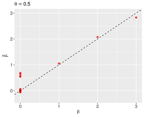
Figure 2: Modal estimates of the regression coefficients

The effect of different $ν_{0}$ and $β^{(0)}$ values on variable selection

Rather than fixing $ν_{0}$ as 0.5, I vary it from 0 to 0.5 to see its effect on the variable selection. I imitate the author’s method to consider the grid of $ν_{0}$ values $V = {0.01 + k \times 0.01 : k = 0, \dots, 50}$ again with $ν_{1} = 1000$ fixed and $β^{(0)} = 1_{p}$ . Figure 3 shows the modal estimates of regression coefficients obtained for each $ν_{0} \in V$ . We can discover that only when $ν_{0} > 0.15$ , we can get a good estimation for the $β$ .I also consider the effect different initial values of $β$ on the variable selection. Fix $ν_{0} = 0.5$ and $ν_{1} = 1000$ , I set the grid of $β^{(0)} = c_{p}$ where $c$ is a p-dimension vector with each value $c_{i} = {- 5 + 0.2 \times k : k = 0, \dots, 50}, i = 1, 2, \dots, p$ . Figure 4 depicts modal estimates of regression coefficients with different initial values of $β^{(0)}$ . We discover only when $| β^{(0)} | < 2$ , we can get good estimation for the $β$ .

I also consider the effect different initial values of $β$ on the variable selection. Fix $ν_{0} = 0.5$ and $ν_{1} = 1000$ , I set the grid of $β^{(0)} = c_{p}$ where $c$ is a p-dimension vector with each value $c_{i} = {- 5 + 0.2 \times k : k = 0, \dots, 50}, i = 1, 2, \dots, p$ . Figure 4 depicts modal estimates of regression coefficients with different initial values of $β^{(0)}$ . We discover only when $| β^{(0)} | < 2$ , we can get good estimation for the $β$ .

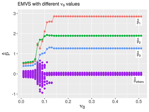
Figure 3: Modal estimates of the regression coefficients

Figure 4: Modal estimates of the regression coefficients

Reference

George, Edward I., and Robert E. McCulloch. 1997. “APPROACHES for Bayesian Variable Selection.” Statistica Sinica 7 (2): 339–73. http://www.jstor.org/stable/24306083.

Rockova, Veronika, and Edward George. 2014. “EMVS: The Em Approach to Bayesian Variable Selection.” Journal of the American Statistical Association 109 (June). https://doi.org/10.1080/01621459.2013.869223.