Bayesian Linear Model

Caleb Jin / 2019-04-18

Linear model

Consider a multiple linear regression model as follows: $y = X β + ϵ,$ where $y = (y_{1}, y_{2}, \dots, y_{n})^{T}$ is the $n$ -dimensional response vector, $X = (x_{1}, x_{2}, \dots, x_{n})^{T}$ is the $n \times p$ design matrix, and $ϵ \sim N_{n} (0, σ^{2} I_{n})$ . We assume that $p < n$ and $X$ is full rank.

Maximum likelihood estimation (MLE) approach

Since $y \sim N_{n} (X β, σ^{2} I_{n})$ , the likelihood function is given as $\begin{array}{rcl} L (β, σ^{2}) & = & f (y | β, σ^{2}) \\ = & (2 π)^{- \frac{n}{2}} | Σ |^{- \frac{1}{2}} \exp {- \frac{1}{2} (y - X β)^{T} Σ^{- 1} (y - X β)}, \end{array}$

where $Σ = σ^{2} I_{n}$ . Then the log likelihood can be written as $\begin{array}{rcl} l (β, σ^{2}) & = & \log L (β, σ^{2}) \\ = & - \frac{n}{2} \log (2 π) - \frac{n}{2} \log (σ^{2}) - \frac{1}{2 σ^{2}} (y - X β)^{T} (y - X β) . \end{array}$ Note that $l (β, σ^{2})$ is a concave function in $(β, σ^{2})$ . Hence, the maximum likelihood estimator (MLE) can be obtained by solving the following equations: $\begin{array}{rcl} \frac{\partial l (β, σ^{2})}{\partial β} & = & - \frac{1}{2 σ^{2}} (- 2 X^{T} y + 2 X^{T} X β) = 0; \\ \frac{\partial l (β, σ^{2})}{\partial σ^{2}} & = & - \frac{n}{2} \frac{1}{σ^{2}} + \frac{1}{2} \frac{1}{(σ^{2})^{2}} (y - X β)^{T} (y - X β) = 0. \end{array}$ Therefore, the MLEs of $β$ and $σ^{2}$ are given as $\begin{array}{rcl} \hat{β} & = & (X^{T} X)^{- 1} X^{T} y; \\ {\hat{σ}}^{2} & = & \frac{(y - X \hat{β})^{T} (y - X \hat{β})}{n} = \frac{‖ y - \hat{y} ‖^{2}}{n}, \end{array}$ where $\hat{y} = X \hat{β}$ .

Distribution of $\hat{β}$ and ${\hat{σ}}^{2}$

Note that if $z \sim N_{k} (μ, Σ)$ , then $A z \sim N_{m} (A μ, A Σ A^{T})$ , where $A$ is an $m \times k$ matrix. Since $y \sim N_{n} (X β, σ^{2} I_{n})$ and $\hat{β} = (X^{T} X)^{- 1} X^{T} y$ , we have $\begin{array}{rcl} \hat{β} & \sim & N_{p} ((X^{T} X)^{- 1} X^{T} X β, σ^{2} (X^{T} X)^{- 1} X^{T} X (X^{T} X)^{- 1}) \\ = & N_{p} (β, σ^{2} (X^{T} X)^{- 1}) . \end{array}$

Note that $y - \hat{y} = (I_{n} - X (X^{T} X)^{- 1} X^{T}) y$ , where $I_{n} - X (X^{T} X)^{- 1} X^{T}$ is an idempotent matrix with rank $(n - p)$ .

$Can you prove that I_{n} - X (X^{T} X)^{- 1} X^{T} s an idempotent matrix of rank (n - p) ?$

Proof. Let $H = X (X^{T} X)^{- 1} X^{T}$ .

$H H = X (X^{T} X)^{- 1} X^{T} X (X^{T} X)^{- 1} X^{T} = X (X^{T} X)^{- 1} X^{T} = H$ thus $H$ is idempotent matrix.

Similarly, as $(I_{n} - H) (I_{n} - H) = I_{n} - H$ , $(I_{n} - H)$ is also idempotent.

Hence we have

r (I_{n} - H) = t r (I_{n} - H) = n - t r (H) = n - t r ((X^{T} X)^{- 1} X^{T} X) = n - p

$How to prove r (I_{n} - H) = t r (I_{n} - H) ?$

The eigenvalue of idempotent matrix is either 1 or 0, hence the rank of it is the sum of eigenvalues, which equals the trace of matrix;

$How to prove trace of matrix is the sum of eigenvalues?$

It requires characteristic polynomial.

Another way to prove this is in this link

From Lemma 1, we have that $\begin{array}{rcl} (1) & n \frac{{\hat{σ}}^{2}}{σ^{2}} \sim χ^{2} (n - p), \end{array}$ where $χ^{2} (n - p)$ denotes the chi-squared distribution with degrees of freedom $n - p$ .

$Can you prove Eq.$ (1)?

Proof. By Lemma 1, we have
$n \frac{{\hat{σ}}^{2}}{σ^{2}} = \frac{{\hat{e}}^{T} \hat{e}}{σ^{2}} = y^{T} (\frac{I_{n} - H}{σ^{2}}) y = y^{T} A y \sim χ^{2} (t r (A Σ), μ^{T} A μ / 2)$

where

A = \frac{I_{n} - H}{σ^{2}}

μ^{T} A μ / 2 = (X β)^{T} (\frac{I_{n} - H}{σ^{2}}) (X β) / 2 = 0

A Σ = (\frac{I_{n} - H}{σ^{2}}) σ^{2} I_{n} = I_{n} - H,

hence

r (A Σ) = n - p

. Therefore

n \frac{{\hat{σ}}^{2}}{σ^{2}} \sim χ^{2} (n - p)

Lemma 1 Let

z \sim N_{k} (μ, Σ)

with

r (Σ) = k

, where

r (Σ)

denotes the rank of

Σ

. If

A Σ

(or

Σ A

) is an idempotent matrix of rank

m

, then

z^{T} A z

follows the non-central chi-squared distribution with degrees of freedom

m

and non-central parameter

λ = μ^{T} A μ / 2

Bayesian approach

$σ^{2}$ is known

Suppose $σ^{2}$ is known. We define the prior distribution of $β$ by $β \sim N_{p} (0, σ^{2} ν I_{p})$ . Then the posterior density of $β$ can be obtained by $\begin{array}{rcl} π (β | y) & \propto & f (y | β) π (β) \\ \propto & \exp (- \frac{1}{2 σ^{2}} ‖ y - X β ‖^{2}) \times \exp (- \frac{1}{2 σ^{2} ν} ‖ β |^{2}) \\ = & \exp [- \frac{1}{2 σ^{2}} {(y - X β)^{T} (y - X β) + \frac{1}{ν} β^{T} β}] \\ \propto & \exp {- \frac{1}{2 σ^{2}} (- 2 β^{T} X^{T} y + β^{T} X^{T} X β + \frac{1}{ν} β^{T} β)} \\ = & \exp {- \frac{1}{2 σ^{2}} (- 2 β^{T} (X^{T} X + \frac{1}{ν} I_{p}) {(X^{T} X + \frac{1}{ν} I_{p})}^{- 1} X^{T} y + β^{T} (X^{T} X + \frac{1}{ν} I_{p}) β)} \\ \propto & \exp {- \frac{1}{2 σ^{2}} (β - \tilde{β})^{T} (X^{T} X + \frac{1}{ν} I_{p}) (β - \tilde{β})} \end{array}$ where $\tilde{β} = {(X^{T} X + \frac{1}{ν})}^{- 1} X^{T} y$ .

This implies that $\begin{array}{rcl} (2) & β | y \sim N_{p} ({(X^{T} X + \frac{1}{ν} I_{p})}^{- 1} X^{T} y, σ^{2} {(X^{T} X + \frac{1}{ν} I_{p})}^{- 1}) . \end{array}$ The Bayesian estimate ${\hat{β}}_{B a y e s} = {(X^{T} X + \frac{1}{ν} I_{p})}^{- 1} X^{T} y$ . It is worth noting that if $ν \to \infty$ , the posterior distribution converges to the distribution of ${\hat{β}}_{M L E} \sim N_{p} (β, σ^{2} (X^{T} X)^{- 1})$ .

$σ^{2}$ is unknown

In general, $σ^{2}$ is unknown. Then, we need to assign a reasonable prior distribution for $σ^{2}$ . We consider the inverse gamma distribution, which is called a , as follows: $σ^{2} \sim I G (a_{0}, b_{0})$ with the density function $\begin{array}{rcl} π (σ^{2}) = \frac{b_{0}^{a_{0}}}{Γ (a_{0})} (σ^{2})^{- a_{0} - 1} \exp (- \frac{b_{0}}{σ^{2}}), \end{array}$ where $a_{0} > 0$ and $b_{0} > 0$ . In addition, we need to introduce prior for $β | σ^{2}$ :

$β | σ^{2} \sim N_{p} (0, σ^{2} ν I_{p}) .$

$Today, we derive the joint posterior distribution π (β, σ^{2} | y) \propto f (y | β, σ) π (β | σ^{2}) π (σ^{2}) .$

Show

1. $π (σ^{2} | β, y) = I G (a^{*}, b^{*})$
1. $π (β | y) \sim$ t-distribution with $t^{*}$

Then the posterior density function of

σ^{2}

given

β, y

can be obtained by

Proof (1). $\begin{array}{rcl} π (σ^{2} | β, y) = \frac{f (y | β, σ^{2}) π (β, σ^{2})}{\int f (y | β, σ^{2}) π (β, σ^{2}) d σ^{2}} = \frac{f (y | β, σ^{2}) π (β | σ^{2}) π (σ^{2})}{\int f (y, β, σ^{2}) d σ^{2}} \\ \propto & f (y | β, σ^{2}) π (β | σ^{2}) π (σ^{2}) \\ \propto & (σ^{2})^{- \frac{n}{2}} \exp (- \frac{1}{2 σ^{2}} ‖ y - X β ‖^{2}) \times (σ^{2})^{- \frac{p}{2}} \exp (- \frac{1}{2 σ^{2} ν} ‖ β ‖^{2}) \times (σ^{2})^{- a_{0} - 1} \exp (- \frac{b_{0}}{σ^{2}}) \\ = & (σ^{2})^{- (\frac{n + p}{2} + a_{0}) - 1} \exp [- \frac{1}{σ^{2}} {\frac{1}{2} ‖ y - X β ‖^{2} + \frac{1}{2 ν} ‖ β ‖^{2} + b_{0}}] \\ = & (σ^{2})^{- a^{*} - 1} \exp (- \frac{b^{*}}{σ^{2}}) \end{array}$ where $a^{*} = \frac{n + p}{2} + a_{0}$ , $b^{*} = \frac{1}{2} ‖ y - X β ‖^{2} + \frac{1}{2 ν} ‖ β ‖^{2} + b_{0}$ .

This implies that

\begin{array}{rcl} σ^{2} | β, y \sim I G (\frac{n + p}{2} + a_{0}, \frac{1}{2} ‖ y - X β ‖^{2} + \frac{1}{2 ν} ‖ β ‖^{2} + b_{0}) . \end{array}

Proof (2). $\begin{array}{rcl} π (β | y) \\ = & \int π (β, σ^{2} | y) d σ^{2} \\ = & \int \frac{f (y | β, σ^{2}) π (β, σ^{2})}{\iint f (y | β, σ^{2}) π (β, σ^{2}) d β d σ^{2}} d σ^{2} \\ \propto & \int f (y | β, σ^{2}) π (β | σ^{2}) π (σ^{2}) d σ^{2} \\ \propto & Γ (a^{*}) b^{- a^{*}} \\ \propto & {b^{*}}^{- a^{*}} \\ = & [\frac{1}{2} ‖ y - X β ‖^{2} + \frac{1}{2 ν} ‖ β ‖^{2} + b_{0}]^{- a^{*}} \\ \propto & {[(y - X β)^{T} (y - X β) + \frac{1}{ν} β^{T} β - 2 b_{0}]}^{- a^{*}} \\ = & {[y^{T} y - 2 β^{T} X^{T} y + β^{T} X^{T} X β + \frac{1}{ν} β^{T} β + 2 b_{0}]}^{- a^{*}} \\ \propto & {[β^{T} (X^{T} X + \frac{1}{ν} I_{p}) β - 2 β^{T} (X^{T} X + \frac{1}{ν} I_{p}) {(X^{T} X + \frac{1}{ν} I_{p})}^{- 1} X^{T} y + y^{T} y + 2 b_{0}]}^{- a^{*}} \\ = & {[β^{T} A β - 2 β^{T} A \tilde{β} + {\tilde{β}}^{T} A \tilde{β} - {\tilde{β}}^{T} A \tilde{β} + y^{T} y + 2 b_{0}]}^{- a^{*}} \\ = & {[(β - \tilde{β})^{T} A (β - \tilde{β}) + y^{T} y - y^{T} X A^{- 1} X^{T} y + 2 b_{0}]}^{- a^{*}} \\ = & {[(β - \tilde{β})^{T} A (β - \tilde{β}) + y^{T} (I_{n} - X A^{- 1} X^{T}) y + 2 b_{0}]}^{- a^{*}} \\ \propto & {[(β - \tilde{β})^{T} A (β - \tilde{β}) + c^{*}]}^{- a^{*}} \\ \propto & {[1 + \frac{1}{c^{*}} (β - \tilde{β})^{T} A (β - \tilde{β})]}^{- \frac{n + p + 2 a_{0}}{2}} \\ = & {[1 + \frac{ν^{*}}{ν^{*} c^{*}} (β - \tilde{β})^{T} A (β - \tilde{β})]}^{- \frac{p + ν^{*}}{2}} \\ = & {[1 + \frac{1}{ν^{*}} (β - \tilde{β})^{T} (\frac{c^{*}}{ν^{*}} A^{- 1})^{- 1} (β - \tilde{β})]}^{- \frac{p + ν^{*}}{2}} \end{array}$ This implies that $\begin{array}{rcl} (3) & β | y \sim M T (\tilde{β}, \frac{c^{*}}{ν^{*}} A^{- 1}, ν^{*}), \end{array}$

where

\begin{array}{rcl} A & = & X^{T} X + \frac{1}{ν} I_{p}, \\ \tilde{β} & = & A^{- 1} X^{T} y, \\ c^{*} & = & y^{T} (I_{n} - X A^{- 1} X^{T}) y + 2 b_{0}, \\ ν^{*} & = & n + 2 a_{0} . \end{array}

Note: the density of a multiple t-distribution with $Σ, μ$ and $ν$ is (3) $\begin{array}{rcl} \frac{Γ [(ν + p) / 2]}{Γ (ν / 2) ν^{p / 2} π^{p / 2} | Σ |^{1 / 2}} {[1 + \frac{1}{ν} (X - μ)^{T} Σ^{- 1} (X - μ)]}^{- (ν + p) / 2} . \end{array}$

Monte Carlo Simulation

Suppose $σ^{2}$ is unknown. If $β \sim N_{p} (0, σ^{2} ν I_{p})$ , we know the distribution of $β | y$ is Eq. (3). According to this known distribution, we can easily compute the $E (β | y)$ and $V (β | y)$ . But in practice, the form of density function $π (β | y)$ is often an unknown and very complicated distribution, leading to be impossible to solve its integration directly. hence we turn to use numerical methods to solve this problem, such as Monte Carlo methods.

For example, a form density function $π (θ | y)$ is an unknown distribution. $E (θ | y) = \int θ π (θ | y) d θ$ . According to lemma , ${\bar{X}}_{n} \to μ = E (X)$ as $n \to \infty$ . Therefore, if we indepedently generate $θ^{(1)}, θ^{(2)}, \dots, θ^{(M)}$ from $π (θ | y)$ , $M^{- 1} \sum_{k = 1}^{M} θ^{(k)} \to E (θ | y)$ as M $\to \infty$ . However, there are two problems.

What if we cannot generate sample from $π (θ | y)$
What if they are not identically and independently distributed.

The solutions to these two question are Monte Carlo (MC) method and Markov Chain Monte Carlo (MCMC).

For the first question, we can use importance sampling method.

Lemma 2 (Strong Law of Large Number)

Let

X_{1}, X_{2}, . . .

be a sequence of i.i.d random variables, each having finite mean m. Then

Pr (lim_{n \to \infty} \frac{1}{n} (X_{1} + X_{2} + . . . + X_{n} = m)) = 1.

$σ^{2}$ is known

Importance Sampling

To estimate mean value of parameters, usually we randomly sample from $π (θ | y)$ and compute their mean value to estimate parameters. However, in practice, it is hard to generate sample directly from $π (θ | y)$ , because we don’t know what speccific distribution it belongs to. hence we return to importance sampling method.

Note that $\begin{array}{rcl} E (θ | y) & = & \int θ π (θ | y) d θ \\ = & \int θ \frac{π (θ | y)}{g (θ)} g (θ) d θ \\ = & \int h (θ) g (θ) d θ \\ = & E {h (θ)} \end{array}$ where $h (θ) = θ \frac{π (θ | y)}{g (θ)}, g (θ)$ is a known pdf.

To estimate the variance of parameters, similarly, $\begin{array}{rcl} V a r (θ | y) & = & E [θ - E (θ | y)]^{2} = \int (θ - E (θ | y))^{2} π (θ | y) d θ \\ = & \int (θ - E (θ | y))^{2} \frac{π (θ | y)}{g (θ)} g (θ) d θ \\ = & \int h^{^{'}} (θ) g (θ) d θ \\ = & E {h^{^{'}} (θ)} \end{array}$ where $h^{^{'}} (θ) = (θ - E (θ | y))^{2} \frac{π (θ | y)}{g (θ)},$ and $g (θ)$ is a known pdf.

The importance sampling method can be implemented as follows:

Note that $\sum_{i = 1}^{M} \frac{h (θ_{i})}{M} \to E (h (θ)) = E (θ | y) . a s M \to \infty$ Estimating variance by importance sampling method is similarly.

Importance Sampling Simulation

Setup

Consider a single linear regression model as follows:

$y_{i} = β_{0} + β_{1} x_{i} + ε_{i}$ where $ε_{i} \sim N (0, 1), x_{i} \sim N (0, 1), β_{0} = 1, β_{1} = 2,$ for $i = 1, \dots, 100.$

We already know that if $β \sim N_{p} (0, σ^{2} ν I_{p})$ , then the distribution of $β | y$ is Eq.(2). Assume $σ = 1$ is known and consider a known pdf $π (β) = ϕ (β; (0, 0), 10 I_{2})$ , hence in this case, $ν = 10$ . Our simulation can be broken down into 3 steps in following:

Find exact value of $E (β_{0} | y), E (β_{1} | y), V (β_{0} | y)$ and $V (β_{1} | y)$
Use the MC method to simulate the results above with size of 100, 1000 and 5000.
Use Importance Sampling Method to simulate relevant results with the same size in (2). Consider the known pdf of parameters are $ϕ (β_{0} | 1, 0.5)$ and $ϕ (β_{1} | 2, 0.5) .$

Simulation Results

We use R softeware to do this simulation.

According to Eq. (2), compute $E (β | y) = {(X^{T} X + \frac{1}{ν} I_{p})}^{- 1} X^{T} y$ and $V a r (β | y) = σ^{2} {(X^{T} X + \frac{1}{ν} I_{p})}^{- 1}$ , where $σ = 1$ and $ν = 10$ , then we get the following results:

$E (β_{0})$ $E (β_{1})$ $V a r (β_{0})$ $V a r (β_{1})$

1.108 1.997 0.01 0.011
Sample directly from normal distribution of Eq. (2) with sample size of 100, 1000 and 5000, then compute the mean and variance values of samples. hence we get the following results:

$E (β_{0})$	$E (β_{1})$	$V a r (β_{0})$	$V a r (β_{1})$
1.108	1.997	0.01	0.011

	$E (β_{0})$	$E (β_{1})$	$V a r (β_{0})$	$V a r (β_{1})$
100	1.104	2.002	0.009	0.012
1000	1.107	1.993	0.011	0.012
5000	1.108	1.996	0.010	0.011

Sample

β_{0}

and

β_{1}

directly from

ϕ (β_{0} | 1, 0.5)

and

ϕ (β_{1} | 2, 0.5)

, respectively, with sample size of 100, 1000 and 5000. And then compute

h (θ_{i})

and

h^{^{'}} (θ_{i})

. Compute mean values of them to get estimates of expectation and variance. The final results are following:

	$E (β_{0})$	$E (β_{1})$	$V a r (β_{0})$	$V a r (β_{1})$
100	1.0500	2.0623	0.0175	0.0127
1000	1.1323	1.9521	0.0106	0.0127
5000	1.1269	2.0478	0.0107	0.0137

$σ^{2}$ is unknown

Suppose $σ^{2}$ is unknown, we cannot use $π (β | y, σ^{2})$ directly.

But we know $π (β, σ^{2} | y) = π (β | y, σ^{2}) π (σ^{2} | y)$ and we already know

$β | y, σ^{2} \sim N_{p} ((X^{T} X + \frac{1}{ν} I_{p})^{- 1} X^{T} y, (X^{T} X + \frac{1}{ν} I_{p})^{- 1} σ^{2})$

So $\begin{array}{rcl} π (σ^{2} | y) = \int π (σ^{2}, β | y) d β \propto \int f (y | σ^{2}, β) π (β | σ^{2}) π (σ^{2}) d β = \int f (y | σ^{2}, β) π (β | σ^{2}) d β \times π (σ^{2}) \\ \propto & \int (σ^{2})^{- \frac{n}{2}} \exp [- \frac{1}{2 σ^{2}} (y - X β)^{T} (y - X β)] (σ^{2})^{- \frac{p}{2}} \exp (- \frac{1}{2 σ^{2} ν} β^{T} β) d β \times π (σ^{2}) \\ \propto & \int \exp [- \frac{1}{2 σ^{2}} (y^{T} y - 2 β^{T} X^{T} y + β^{T} X^{T} X β + \frac{1}{ν} β^{T} β)] d β ((σ^{2})^{- \frac{1}{2} (n + p)} π (σ^{2})) \\ = & \int \exp [- \frac{1}{2 σ^{2}} (β^{T} (X^{T} X + \frac{1}{ν} I_{p}) β - 2 β^{T} (X^{T} X + \frac{1}{ν} I_{p}) (X^{T} X + \frac{1}{ν} I_{p})^{- 1} X^{T} y + y^{T} y)] d β \\ ((σ^{2})^{- \frac{1}{2} (n + p)} π (σ^{2})) \\ = & \int \exp [- \frac{1}{2 σ^{2}} (β - \tilde{β})^{T} A (β - \tilde{β}) + y^{T} y - {\tilde{β}}^{T} A \tilde{β}] d β ((σ^{2})^{- \frac{1}{2} (n + p)} π (σ^{2})) \\ = & \int \exp [- \frac{1}{2 σ^{2}} (β - \tilde{β})^{T} A (β - \tilde{β})] d β \times \exp [- \frac{1}{2 σ^{2}} (y^{T} y - y^{T} X A^{- 1} X^{T} y)] ((σ^{2})^{- \frac{1}{2} (n + p)} π (σ^{2})) \\ = & (2 π)^{\frac{p}{2}} | σ^{2} A^{- 1} |^{\frac{1}{2}} \exp [- \frac{1}{2 σ^{2}} (y^{T} (I_{n} - X A^{- 1} X^{T}) y)] ((σ^{2})^{- \frac{1}{2} (n + p)} π (σ^{2})) \\ \propto & (σ^{2})^{\frac{p}{2} - \frac{1}{2} (n + p)} (σ^{2})^{- a_{0} - 1} \exp [- \frac{1}{σ^{2}} (b_{0} + \frac{1}{2} y^{T} (I_{n} - X A^{- 1} X^{T}) y)] \\ = & (σ^{2})^{- (\frac{1}{2} n + a_{0}) - 1} \exp [- \frac{1}{σ^{2}} (b_{0} + \frac{1}{2} y^{T} (I_{n} - X A^{- 1} X^{T}) y)] \\ = & (σ^{2})^{- a^{*} - 1} \exp (- \frac{b^{*}}{σ^{2}}) \end{array}$ where $A = (X^{T} X + \frac{1}{ν} I_{p}), \tilde{β} = A^{- 1} x^{T} y, a^{*} = \frac{1}{2} n + a_{0}, b^{*} = b_{0} + \frac{1}{2} y^{T} (I_{n} - X A^{- 1} X^{T}) y$ .

This is proportional to the pdf of $I G (a^{*}, b^{*})$ . Hence we have $\begin{array}{rcl} E (β | y) & = & \int β π (β | y) d β = \int β [\int π (β, σ^{2} | y) d σ^{2}] d β \\ = & \int \int β [π (β | y, σ^{2}) π (σ^{2} | y) d σ^{2}] d β, \end{array}$ Similarly, $\begin{array}{rcl} V a r (β | y) & = & \int (β - E (β | y)) π (β | y) d β = \int (β - E (β | y)) [\int π (β, σ^{2} | y) d σ^{2}] d β \\ = & \int \int (β - E (β | y)) [π (β | y, σ^{2}) π (σ^{2} | y) d σ^{2}] d β, \end{array}$

Plug-in Sampling Method

We can estimate mean of $β$ by computing $E (β | y) = \sum_{m = 1}^{M} β^{(m)} / M$ , where $β^{(m)}$ are generaed as follows:

1. Generate $σ^{2 (m)}$ from $π (σ^{2} | y)$ , where $σ^{2} | y$ is from $I G (a^{*}, b^{*})$
1. For given $σ^{2 (m)}$ , generate $β^{(m)}$ from $π (β | y, σ^{2 (m)})$ , where it is from normal distribution in Eq. (2)

Simulation Results

We use the same setup in the Section Importance Sampling Simulation. The final result is as follows:

	$E (β_{0})$	$E (β_{1})$	$V a r (β_{0})$	$V a r (β_{1})$
100	1.1099	1.9960	0.0073	0.0107
1000	1.1049	2.0004	0.0079	0.0084
5000	1.1081	1.9966	0.0081	0.0088

Markov Chain Monte Carlo Simulation

Gibbs Samping

Suppose $σ^{2}$ is unknown, we know $σ^{2} | y, β_{0}, β_{1} \sim I G (a^{*}, b^{*})$ $β | y, σ^{2} \sim N_{p} ((X^{T} X + \frac{1}{ν} I_{p})^{- 1} X^{T} y, (X^{T} X + \frac{1}{ν} I_{p})^{- 1} σ^{2})$ hence we can get the conditional distribution of each parameter, $β_{0} | β_{1}, y, σ^{2} \sim N (μ_{0} + \frac{σ_{0}}{σ_{1}} ρ (β_{1} - μ_{1}), (1 - ρ^{2}) σ_{1}^{2})$ $β_{1} | β_{0}, y, σ^{2} \sim N (μ_{1} + \frac{σ_{1}}{σ_{0}} ρ (β_{0} - μ_{0}), (1 - ρ^{2}) σ_{0}^{2})$ where $σ_{0} = [1, 0] A^{- 1} σ^{2} [1, 0]^{T}$ , $σ_{1} = [0, 1] A^{- 1} σ^{2} [0, 1]^{T}$ , $μ_{0} = A^{- 1} X^{T} y [1, 0]^{T}$ and $μ_{1} = A^{- 1} X^{T} y [0, 1]^{T}$ .

To generate $β^{(m)}$ from $π (β | y)$ , we can use a MCMC method of Gibbs sampling. The Gibbs sampling, which is one of the most popular MCMC methods, can be implemented as follows:

Set the initial value $(β_{0}^{(0)}, β_{1}^{(0)}, σ^{2 (0)})$ . Then iterate the following steps for $t = 0, 1, 2, \dots$ .

Step1: Generate $σ^{2 (t + 1)}$ from $π (σ^{2} | y, β_{0}^{(t)}, β_{1}^{(t)})$ .

Step2: Generate $β_{0}^{(t + 1)}$ from $π (β_{0} | y, β_{1}^{(t)}, σ^{2 (t + 1)})$ .

Step3: Generate $β_{1}^{(t + 1)}$ from $π (β_{1} | y, β_{0}^{(t + 1)}, σ^{2 (t + 1)})$ .

We setup the total sample size is 5000, and burning period is 2000.

The final result is as follows:

	$E (β_{0})$	$E (β_{1})$	$V a r (β_{0})$	$V a r (β_{1})$
5000	1.1096	1.9955	0.0082	0.009

The diagnosis tool to assess the convergence of the sampler is as follows:

$$\beta_0$; $\beta_1$; the marginals and the joint distribution$ $$\beta_0$; $\beta_1$; the marginals and the joint distribution$ $$\beta_0$; $\beta_1$; the marginals and the joint distribution$

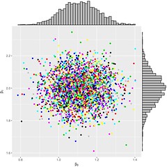
Figure 1: $β_{0}$ ; $β_{1}$ ; the marginals and the joint distribution

Bayesian V.S. Frequentist Case Study

Multivariable Normal Conditional Distribution

The conditional posterior of $β_{j}$ is obtained as follows: $\begin{array}{rcl} π (β_{j} | β_{- j}, σ^{2}, y) & \propto & π (β_{j}, β_{- j} | σ^{2}, y) \\ = & π (β | σ^{2}, y) \\ \propto & f (β, y | σ^{2}) \\ = & f (y | β, σ^{2}) π (β | σ^{2}) \\ \propto & \exp (- \frac{1}{2 σ^{2}} ∥ y - X β ∥^{2}) \exp (- \frac{1}{2 σ^{2} ν} ∥ β ∥^{2}) \\ \propto & \exp [- \frac{1}{2 σ^{2}} ((y - X_{- j} β_{- j} - x_{j} β_{j})^{T} (y - X_{- j} β_{- j} - x_{j} β_{j}) + \frac{1}{ν} β_{j}^{T} β_{j})] \\ \propto & \exp [- \frac{1}{2 σ^{2}} (- y^{T} x_{j} β_{j} + β_{- j}^{T} X_{- j}^{T} x_{j} β_{j} - β_{j}^{T} x_{j}^{T} y + β_{j}^{T} x_{j}^{T} X_{- j} β_{- j} + β_{j}^{T} x_{j}^{T} x_{j} β_{j} + \frac{1}{ν} β_{j}^{T} β_{j})] \\ \propto & \exp [- \frac{1}{2 σ^{2}} (- 2 β_{j}^{T} x_{j}^{T} y + 2 β_{j}^{T} x_{j}^{T} X_{- j} β_{- j} + β_{j}^{T} x_{j}^{T} x_{j} β_{j} + \frac{1}{ν} β_{j}^{T} β_{j})] \\ = & \exp [- \frac{1}{2 σ^{2}} (β_{j}^{T} (x_{j}^{T} x_{j} + \frac{1}{ν}) β_{j} - 2 β_{j}^{T} x_{j}^{T} (y - X_{- j} β_{- j}))] \\ = & \exp [- \frac{1}{2 σ^{2}} (x_{j}^{T} x_{j} + \frac{1}{ν}) (β_{j}^{T} β_{j} - 2 β_{j}^{T} (x_{j}^{T} x_{j} + \frac{1}{ν})^{- 1} x_{j}^{T} (y - X_{- j} β_{- j}))] \\ = & \exp [- \frac{1}{2 σ^{2}} (x_{j}^{T} x_{j} + \frac{1}{ν}) (β_{j} - {\tilde{β}}_{j})^{2}] \end{array}$ where ${\tilde{β}}_{j} = (x_{j}^{T} x_{j} + \frac{1}{ν})^{- 1} x_{j}^{T} (y - X_{- j} β_{- j})$ , $X_{- j}$ is a submatrix of $X$ without the $j^{t h}$ column, and $β_{- j}$ is a subvector of $β$ without the $j^{t h}$ element. Hence

$β_{j} | β_{- j}, σ^{2}, y \sim N ((x_{j}^{T} x_{j} + \frac{1}{ν})^{- 1} x_{j}^{T} (y - X_{- j} β_{- j}), σ^{2} {[x_{j}^{T} x_{j} + \frac{1}{ν}]}^{- 1})$

Setup

Consider

$f (y | β, σ^{2}) = (2 π σ^{2})^{- \frac{n}{2}} \exp (- \frac{1}{2 σ^{2}} ∥ y - X β ∥^{2}),$ $π (β | σ^{2}) = (2 π σ^{2} ν)^{- \frac{p}{2}} \exp (- \frac{1}{2 σ^{2} ν} ∥ β ∥^{2}) .$

Generate 30 samples from $y = 1 + 1 \times x_{1} + 2 \times x_{2} + 0 \times x_{3} + 0 \times x_{4} + 10 \times x_{5} + ϵ$ where $ϵ \sim N (0, 2), x_{i} \sim N (0, 1) . β = (1, 1, 2, 0, 0, 10)$

use frequentist way method to estimate $β$
use Bayesian MC
use Bayesian MCMC

Computation Algorithm

In frequentist way, that is OLS method, we know the estimate of $β$ is $\hat{β} = (X^{T} X)^{- 1} X^{T} y$ . The mean square of error is $∥ \hat{β} - β ∥^{2} / 6$ .
In Bayesian MC way, we assume that

$σ^{2} \sim I G (a_{0}, b_{0})$

$β | σ^{2} \sim N (0, σ^{2} ν I_{p})$

Then we have proved that

$σ^{2} | y \sim I G (a^{*}, b^{*})$ , where $a^{*} = \frac{n}{2} + a_{0}, b^{*} = b_{0} + \frac{1}{2} y^{T} (I_{n} - X A^{- 1} X^{T}) y$

$β | y, σ^{2} \sim N (A^{- 1} X^{T} y, A^{- 1} σ^{2})$ , where $A = (X^{T} X + \frac{1}{ν} I_{p})$

hence

β^{(m)}

are generaed as follows:

Finally, we estimate $\hat{β}$ by computing $E (β | y) = \sum_{m = 1}^{M} β^{(m)} / M$ . The mean square of error is $∥ \hat{β} - β ∥^{2} / 6$ .

In Bayesian MCMC way, we have proved that
1. $σ^{2} | y, β \sim I G (a^{*}, b^{*})$ , where $a^{*} = \frac{n + p}{2} + a_{0}, b^{*} = b_{0} + \frac{1}{2} ∥ y - X β ∥^{2} + \frac{1}{2 ν} ∥ β ∥^{2}$
1. $β | y, σ^{2} \sim N (A^{- 1} X^{T} y, A^{- 1} σ^{2})$ ,where $A = (X^{T} X + \frac{1}{ν} I_{p})$
1. $β_{j} | β_{- j}, σ^{2}, y \sim N ((x_{j}^{T} x_{j} + \frac{1}{ν})^{- 1} x_{j}^{T} (y - X_{- j} β_{- j}), σ^{2} {[x_{j}^{T} x_{j} + \frac{1}{ν}]}^{- 1})$

Then, we use Gibbs sampling method to get the $β^{(m)} = (β_{0}^{(m)}, β_{1}^{(m)}, \dots, β_{5}^{(m)})$ . Set the initial values $(β_{0}^{(0)}, β_{1}^{(0)}, \dots, β_{5}^{(0)}, σ^{2 (0)})$ .Then iterate the following steps for $t = 0, 1, 2, \dots$ as follows:

1. Generate $σ^{2 (t + 1)}$ from $π (σ^{2} | y, β_{0}^{(t)}, β_{1}^{(t)}, \dots, β_{5}^{(t)})$ .
1. Generate $β_{0}^{(t + 1)}$ from $π (β_{0} | y, β_{- 0}^{(t)}, σ^{2 (t + 1)})$ .
1. update $β^{(t)}$ with $β^{(t)} = (β_{0}^{(t + 1)}, β_{1}^{(t)}, \dots, β_{5}^{(t)})$
1. Generate $β_{1}^{(t + 1)}$ from $π (β_{1} | y, β_{- 1}^{(t)}, σ^{2 (t + 1)})$ .
1. update $β^{(t)}$ with $β^{(t)} = (β_{0}^{(t + 1)}, β_{1}^{(t + 1)}, β_{2}^{(t)}, \dots, β_{5}^{(t)})$ and similarly, generate $β_{2}^{(t + 1)}, \dots, β_{5}^{(t + 1)}$ and update $β^{(t)}$ after generating $β_{i}^{(t + 1)}$ every time,

where $β_{- i}^{(t)}$ is a subvector of $β$ without $i^{t h}$ element.

We setup the total sample size is 5000, and burning period is 2000.

Finally, we estimate $\hat{β}$ by computing $E (β | y) = \sum_{m = 2001}^{M} β^{(m)} / M$ . The mean square of error is $∥ \hat{β} - β ∥^{2} / 6$ .

Simulation Results

Bayesian V.S. Frequentist
	$β_{0}$	$β_{1}$	$β_{2}$	$β_{3}$	$β_{4}$	$β_{5}$	MSE
Frequentist	1.194	0.991	2.080	-0.082	-0.051	9.608	0.035
Bayesian MC	1.195	0.972	2.084	-0.090	-0.068	9.570	0.041
Bayesian MCMC	1.187	0.986	2.071	-0.085	-0.058	9.581	0.038

Model Selection

Consider we have k candidate models, $M = {M_{1}, M_{2}, \dots, M_{k}}$ . A Bayesian way to select the best model is to find the model which maximizes the model posterior probability given data, that is

$\hat{M} = \arg max_{M \in M} π (M | y)$ where $π (M | y) = \frac{f (y | M) π (M)}{\sum_{\tilde{M} \in M} f (y | \tilde{M}) π (\tilde{M})}$ in which, the denominator is free of $M$ . note that the prior $π (M) = 1 / k$ . Then we have $π (M | y) = \frac{f (y | M)}{\sum_{w \in M} f (y | \tilde{M})}$ This leads to $\hat{M} = \arg max_{M \in M} f (y | M)$ where $f (y | M) = \int f (y | θ_{M}, M) π (θ_{M}) d θ_{M}$ , where $θ_{M}$ is the parameter under model $M$ . We call $f (y | M)$ as marginal likelihood under model $M$ , $f (y | θ_{M}, M)$ likelihood under model $M$ and $π (θ_{M})$ prior under model M. Under $M$ $\begin{array}{rcl} f (y | M) & = & \int f (y | θ, M) π (θ | M) d θ \\ = & \int \int f (y | β, σ^{2}, M) π (β | σ^{2}, M) π (σ^{2} | M) d β d σ^{2} \\ = & \int \int (2 π)^{- \frac{n}{2}} (σ^{2})^{- \frac{n}{2}} \exp [- \frac{1}{2 σ^{2}} (y - X β_{M})^{T} (y - X β_{M})] \times \\ (2 π)^{- \frac{p_{M}}{2}} (σ^{2} ν)^{- \frac{p_{M}}{2}} \exp (- \frac{1}{2 σ^{2} ν} β_{M}^{T} β_{M}) \times \\ \frac{b_{1}^{a_{1}}}{Γ (a_{1})} (σ^{2})^{(- a_{1} - 1)} \exp (- \frac{b_{1}}{σ^{2}}) d β_{M} d σ^{2} \\ = & \frac{b_{1}^{a_{1}}}{Γ (a_{1}) ν^{\frac{p_{M}}{2}}} (2 π)^{(- \frac{n + p_{M}}{2})} \int \int σ^{2 (\frac{- (n + p_{M} + 2 a_{1} + 2)}{2})} \times \\ \exp [- \frac{1}{2 σ^{2}} (y^{T} y - 2 β_{M}^{T} X^{T} y + β_{M}^{T} X^{T} X β_{M} + \frac{1}{ν} β_{M}^{T} β_{M} + 2 b_{1})] d β_{M} d σ^{2} \end{array}$ Note that $\begin{array}{rcl} y^{T} y - 2 β_{M}^{T} X^{T} y + β_{M}^{T} X^{T} X β_{M} + \frac{1}{ν} β_{M}^{T} β_{M} + 2 b_{1} \\ = & β_{M}^{T} (X^{T} X + \frac{1}{ν} I_{p_{M}}) β_{M} - 2 β_{M}^{T} (X^{T} X + \frac{1}{ν} I_{p_{M}}) {(X^{T} X + \frac{1}{ν} I_{p_{M}})}^{- 1} X^{T} y + y^{T} y + 2 b_{1} \\ = & β_{M}^{T} A β_{M} - 2 β_{M}^{T} A \tilde{β_{M}} + {\tilde{β_{M}}}^{T} A \tilde{β_{M}} - {\tilde{β_{M}}}^{T} A \tilde{β_{M}} + y^{T} y + 2 b_{1} \\ = & (β_{M} - \tilde{β_{M}})^{T} A (β - \tilde{β_{M}}) + y^{T} y - y^{T} X A^{- 1} X^{T} y + 2 b_{1} \\ = & (β_{M} - \tilde{β_{M}})^{T} A (β_{M} - \tilde{β_{M}}) + y^{T} (I_{n} - X A^{- 1} X^{T}) y + 2 b_{1} \end{array}$ Therefore, $\begin{array}{rcl} f (y | M) & = & \frac{b_{1}^{a_{1}}}{Γ (a_{1}) ν^{\frac{p_{M}}{2}}} (2 π)^{(- \frac{n + p_{M}}{2})} \int \int σ^{2 (\frac{- (n + p_{M} + 2 a_{1} + 2)}{2})} \times \\ \exp [- \frac{1}{2 σ^{2}} ((β_{M} - \tilde{β_{M}})^{T} A (β_{M} - \tilde{β_{M}}) + y^{T} (I_{n} - X A^{- 1} X^{T}) y + 2 b_{1})] d β_{M} d σ^{2} \\ = & \frac{b_{1}^{a_{1}}}{Γ (a_{1}) ν^{\frac{p_{M}}{2}}} (2 π)^{(- \frac{n + p_{M}}{2})} \int σ^{2 (\frac{- (n + p_{M} + 2 a_{1} + 2)}{2})} \times \\ (2 π)^{\frac{p_{M}}{2}} | A |^{- \frac{1}{2}} \exp [- \frac{1}{2 σ^{2}} (y^{T} (I_{n} - X A^{- 1} X^{T}) y + 2 b_{1})] d σ^{2} \\ = & \frac{b_{1}^{a_{1}}}{Γ (a_{1}) ν^{\frac{p_{M}}{2}}} (2 π)^{(- \frac{n}{2})} | A |^{- \frac{1}{2}} \int σ^{2 (- a_{M}^{*} - 1)} \exp (- \frac{b_{M}^{*}}{σ^{2}}) d σ^{2} \\ = & \frac{b_{1}^{a_{1}}}{Γ (a_{1}) ν^{\frac{p_{M}}{2}}} (2 π)^{(- \frac{n}{2})} | A |^{- \frac{1}{2}} Γ (a_{M}^{*}) b_{M}^{* (- a_{M}^{*})} \\ = & (2 π)^{(- \frac{n}{2})} \frac{Γ (a_{M}^{*}) b_{M}^{* (- a_{M}^{*})} b_{1}^{a_{1}}}{Γ (a_{1}) ν^{\frac{p_{M}}{2}}} | A |^{- \frac{1}{2}} \end{array}$ where $\begin{array}{rcl} A & = & X^{T} X + \frac{1}{ν} I_{p_{M}}, \tilde{β_{M}} = A^{- 1} X^{T} y \\ a_{M}^{*} & = & \frac{n + p_{M}}{2} + a_{1}, b_{M}^{*} = \frac{1}{2} y^{T} (I_{n} - X A^{- 1} X^{T}) y + b_{1} \end{array}$ After Laplace approximation, $f (y | M)$ is equivalent to BIC for large n.

MCMC

Minghui Chen (IWDE)

Goal is to compute $m (y) = \int f (y | θ) π (θ) d θ$

$\begin{array}{rcl} π (θ | y) = \frac{f (y | θ) π (θ)}{\int f (y | θ) π (θ) d θ} \end{array}$ Let $g (θ)$ be a density function of $θ$

Then,

$\begin{array}{rcl} \int g (θ) d θ = 1 \\ \Leftrightarrow & \int g (θ) \frac{π (θ | y)}{π (θ | y)} d θ = 1 \\ \Leftrightarrow & \int g (θ) \frac{π (θ | y)}{\frac{f (y | θ) π (θ)}{m (y)}} d θ = 1 \\ \Leftrightarrow & m (y) \int \frac{g (θ)}{f (y | θ) π (θ)} π (θ | y) d θ = 1 \\ \Leftrightarrow & m (y) = {[\int \frac{g (θ)}{f (y | θ) π (θ)} π (θ | y) d θ]}^{- 1} \\ = E {[\frac{g (θ)}{f (y | θ) π (θ)} | y]}^{- 1} \\ \approx {[\sum_{m = 1}^{M} \frac{g (θ^{(m)})}{f (y | θ^{(m)}) π (θ^{(m)})} / M]}^{- 1} \end{array}$ where $θ^{(m)}$ is from $π (θ | y)$ .

There maxmimum of $m (y)$ is equivalent to maximize $E {[\frac{g (θ)}{f (y | θ) π (θ)} | y]}^{- 1}$

Now let’s use Minghui Chen’s method to maximize the $f (y | M_{i})$ .

$f (y | M_{i}) = \int f (y | θ, M_{i}) π (θ | M_{i}) d θ$ , where $θ = (β_{0}, β_{1}, σ^{2})$ $\begin{array}{rcl} π (θ | y, M_{i}) & = & \frac{f (y | θ, M_{i}) π (θ | M_{i})}{\int f (y | θ, M_{i}) π (θ | M_{i}) d θ} \\ = & \frac{f (y | θ, M_{i}) π (θ | M_{i})}{f (y | M_{i})} \end{array}$ Let $g (θ)$ be a density function of $θ$

Then

$\begin{array}{rcl} \int g (θ) d θ = 1 \\ \Leftrightarrow & \int g (θ) \frac{π (θ | y, M_{i})}{π (θ | y, M_{i})} d θ = 1 \\ \Leftrightarrow & \int g (θ) \frac{π (θ | y, M_{i})}{\frac{f (y | θ, M_{i}) π (θ | M_{i})}{f (y | M_{i})}} d θ = 1 \\ \Leftrightarrow & f (y | M_{i}) \int \frac{g (θ)}{f (y | θ, M_{i}) π (θ | M_{i})} π (θ | y, M_{i}) d θ = 1 \\ \Leftrightarrow & f (y | M_{i}) = {[\int \frac{g (θ)}{f (y | θ, M_{i}) π (θ | M_{i})} π (θ | y, M_{i}) d θ]}^{- 1} \\ = E {[\frac{g (θ)}{f (y | θ, M_{i}) π (θ | M_{i})} | y, M_{i}]}^{- 1} \\ \approx {[\sum_{n = 1}^{N} \frac{g (θ^{(n)})}{f (y | θ^{(n)}, M_{i}) π (θ^{(n)} | M_{i})} / N]}^{- 1} \end{array}$ where $θ^{(n)}$ is from $π (θ | y, M_{i}), i = 1, 2, \dots, k$ .

The issue here is a choice of $g (θ)$ to minimize MC error.

Recall $π (θ | y) \propto f (y | θ) π (θ) \approx g (θ)$ Let $g (θ)$ be a normal density such that $E_{g} (θ) =$ posterior mean $\approx \sum_{m = 1}^{M} θ^{(m)} / M = \bar{θ}$ , $V_{g} (θ) =$ posterior variance matrix $\approx \sum_{m = 1}^{M} (θ^{(m)} - \bar{θ}) (θ^{(m)} - \bar{θ})^{T} / M$ , where $θ^{(m)}$ is a MCMC sample from $π (θ | y)$ .

For given model M, using MCMC, generate $θ_{M}^{(k)}$ from $π (θ_{M} | y, M)$ , then compute ${\bar{θ}}_{M}$ and $V_{M}$ .

Define $g (θ | M) = N (θ; {\bar{θ}}_{M}, V_{M})$ .

Compute

$\begin{array}{rcl} (4) & f (y | M) \approx {[\sum_{k = 1}^{K} \frac{g (θ^{(k)} | M)}{f (y | θ^{(k)}, M) π (θ^{(k)} | M)} / K]}^{- 1} \end{array}$

Bayesian Simulation Case Study

Setup

Consider

Generate 30 samples from $y = 1 + 1 \times x_{1} + 2 \times x_{2} + 0 \times x_{3} + 0 \times x_{4} + 10 \times x_{5} + ϵ$ where $ϵ \sim N (0, 2), x_{i} \sim N (0, 1) . β = (1, 1, 2, 0, 0, 10)$

Therefore, the true model, say $M_{t u r e}$ , is $y = 1 + 1 \times x_{1} + 2 \times x_{2} + 10 \times x_{5} + ϵ$

1. use Bayesian MC method to find true model
1. use frequentist way method to find true model

Our candidate models are as follows: $M_{1} : y = β_{0} + ϵ;$ $M_{2} : y = β_{0} + β_{1} X_{1} + ϵ;$ $\dots$ $M_{32} : y = 1 + 1 \times x_{1} + 2 \times x_{2} + 0 \times x_{3} + 0 \times x_{4} + 10 \times x_{5} + ϵ$

For bayesian way, compute

$f (y | M_{k})$ for $k = 1, 2, \dots, 32$ and select the best model $\hat{M}$ , such that $f (y | \hat{M}) \geq f (y | M_{k})$ If $\hat{M} = M_{t r u e}$ , then assign $Z_{i} = 1$ , otherwise $Z_{i} = 0$ .

Repeat the above procedure for $R = 500$ times, and compute $\sum_{i = 1}^{R} \frac{Z_{i}}{R} ≃ P ($ selecting true model with Bayes method $)$ .

For Frequentist way, similarly, build linear model for 32 candidate models, compute AIC and BIC. If the smallest AIC or BIC is ture model, then $W_{i} = 1$ , otherwise $W_{i} = 0$ . Repeat it 500 times and compute $\sum_{i = 1}^{R} \frac{W_{i}}{R}$ .

Consider the sample sizes are 20, 50, 100 and 300 so that we can see how sample size impacts the probability of selecting the true model.

For MCMC, sampling with MCMC method, then compute Eq. (4) for 32 candidates models, select the best model $\hat{M}$ , such that $f (y | \hat{M}) \geq f (y | M_{k})$ If $\hat{M} = M_{t r u e}$ , then assign $Z_{i} = 1$ , otherwise $Z_{i} = 0$

Repeat the above procedure for $R = 500$ times, and compute $\sum_{i = 1}^{R} \frac{Z_{i}}{R} ≃ P ($ selecting true model with MCMC method $)$

Result

	MC	AIC	BIC	MCMC	Error
20	0.502	0.560	0.656	0.508	59.401
50	0.894	0.668	0.882	0.880	78.224
100	0.998	0.676	0.916	0.926	93.176
300	0.998	0.712	0.978	NA	NA

Linear model

Maximum likelihood estimation (MLE) approach

Distribution of ^ββ^ and ^σ2σ^2

Bayesian approach

σ2σ2 is known

σ2σ2 is unknown

Monte Carlo Simulation

σ2σ2 is known

Importance Sampling

Importance Sampling Simulation

σ2σ2 is unknown

Plug-in Sampling Method

Simulation Results

Markov Chain Monte Carlo Simulation

Bayesian V.S. Frequentist Case Study

Multivariable Normal Conditional Distribution

Setup

Computation Algorithm

Simulation Results

Model Selection

Model Selection

MCMC

Bayesian Simulation Case Study

Distribution of $\hat{β}$ and ${\hat{σ}}^{2}$

$σ^{2}$ is known

$σ^{2}$ is unknown

$σ^{2}$ is known

$σ^{2}$ is unknown