k-Nearst Neighbor (k-NN)
2020-04-04
General Introduction
\(k\)-Nearest Neighbor (\(k\)-NN) is a basic classification and regression method.
What questions is \(k\)-NN gonna solve?
Ex: Consider the Fig. 1 illustrating a dataset with the coordinates of \(({\bf X}, {\bf y}) = (\{{\bf x}_1,{\bf x}_2\}, {\bf y})\): \((\{3,3\},\text{Blue}), (\{6,2\},\text{Red}), \ldots, (\{4,5\},\text{Blue})\), then what is the category for green dot with \((\{5,3\},{\color{red}{?}})\)
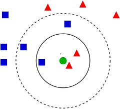
Figure 1: Classifying the green dot
Thus, the \(k\)-NN solves problems like this: the input of \(k\)-NN is the feature vector from the feature space, and the output is the class of the feature vector. For a new feature, the output is decided by majority voting.
Basic idea described in wiki: In \(k\)-NN classification, an object is classified by a plurality vote of its neighbors, with the object being assigned to the class most common among its \(k\) nearest neighbors (\(k\) is a positive integer, typically small).
Three elements in \(k\)-NN Model
A \(k\)-NN model consists of three basic elements: distance, \(k\)-value, and the classification rule.
Distance Metric
Distance Metric: The distance between two points in the feature space measures the similarity/dissimilarity between these two points.
Quantificaton: \(k\)-NN requires all the features should be quantified. If the feature includes color like in Fig. 1, the color can be converted to RGB values to realize the measurement of the distance.
Normalization: Features with larger values assign a larger influence than the smaller values. Thus, features should be normalized before being training.
Suppose \({\bf x}_i,{\bf x}_j\in\mathscr{X}\subseteq\mathbb{R}^d\) with \[ {\bf x}_i = (x_i^{(1)},x_i^{(2)},\ldots,x_i^{(d)})^{{\top}}, {\bf x}_j = (x_j^{(1)},x_j^{(2)},\ldots,x_j^{(d)})^{{\top}}. \] The \(L_p\)-distance (Minkowski distance) of \({\bf x}_i\) and \({\bf x}_j\) is defined as \[ L_p({\bf x}_i,{\bf x}_j) = \left(\sum_{l=1}^{d}|x_i^{(l)}-x_j^{(l)}|^p \right)^{1/p}. \] The \(L_p\)-distance (Minkowski distance) reduces to
Euclidean distance when \(p=2\).
Manhattan distance when \(p=1\).
Chebyshev distance \(L_{\infty}({\bf x}_i,{\bf x}_j) = \max_l|x_i^{(l)}-x_j^{(l)}|\) when \(p=\infty\).
\(k\)-value
When tested with a new example, it looks through the whole training dataset to find \(k\) training examples that are closest to the new example. \(k\) is therefore just the number of neighbors “voting” on the test example’s class.
The choice of \(k\).
When \(k\) is small, the object is assigned by less number of its neighbor. When \(k=1\), \(k\)-NN is called nearest neighbor algorithm. The new example is assigned to the class of its nearest neighbor.
Only closed neighbors vote for the prediction.
The classifier is sensitive to its closed neighbors that increases the estimate error.
It is prone to overfitting and leads to more complex models.
If the closed instants are accidently noise, the prediction is wrong.
When \(k\) is large, the object is classified by larger number of its neighbors. When \(k=N\), the object is classified to the class that has largest proportion in the feature space.
Large \(k\) reduces effect of the noise on the classification and decrease the estimate error of “learning”.
Large \(k\) is prone to have simpler models, and too large \(k\) makes model too simpler, ignoring the useful information in the training instances.
Cross-validation is often used for choosing \(k\)-values.
Classification Rule: Strategy
The commonly used decision rule is majority voting, which is equivalent to minimizer of emperical risk function.
Suppose the loss function is \(0-1\) loss, we define
Classification function is \(f:\mathbb{R}^n\rightarrow c_j\in\{c_1,c_2,\ldots,c_K\}\), and
Misclassification probability is \(P(Y\neq f({\bf x}) = 1-P(Y=f({\bf x}))\)
Suppose any instance \({\bf x}\in\mathscr{X}\), denote \(N_k({\bf x})\) as \(k\) instances in its \(k\)-NN. Assume \(N_k({\bf x})\) contains a class \(c_j\) (\(c_j\in\{c_1,c_2,\ldots,c_K\}\) is unknown yet), then the misclassification rate is \[\begin{eqnarray} \frac{1}{k}\sum_{{\bf x}_i\in N_k(x)}\mathbb{I}(y_i\neq c_j) = 1 - \frac{1}{k}\sum_{{\bf x}_i\in N_k(x)}\mathbb{I}(y_i= c_j).\tag{1} \end{eqnarray}\] misclassification rate is emperical risk function in the training data. To minimize Eq. (1) is equivalent to minimize emperical risk function, thus it is maximizer of majority voting: \[ c = \arg\max_{c_j\in\{c_1,c_2,\ldots,c_K\}}\sum_{{\bf x}_i\in N_k(x)}\mathbb{I}(y_i= c_j). \]
\(k\)-NN Algorithm
Input:
Training data \(\mathscr{T} = ({\bf x}_1,y_1), ({\bf x}_2,y_1),\ldots,({\bf x}_n,y_n), {\bf x}_i\in\mathscr{X}\subseteq\mathbb{R}^n\), \(y_i\in\mathscr{Y} = \{c_1,c_2,\ldots,c_K\}\).
New feature vector \({\bf x}\).
Output:
- The class of \(y\) of \({\bf x}\).
Steps:
According to the given distance metric, find the \(k\)-NN points of \({\bf x}\in\mathscr{T}\). Denote this neighbor as \(N_k({\bf x})\).
Decide the class of \({\bf x}\) according to the majority voting principle in \(N_k({\bf x})\):
\[ y = \arg\max_{c_j\in\mathscr{Y}}\sum_{{\bf x}_i\in N_k(x)}\mathbb{I}(y_i= c_j), \] where \(i = 1,2,\ldots,n;j = 1,2,\ldots,K\).
\(kd\) tree (\(k\)-dimensional tree)
*linear scan**: The most straightforward way to determine the \(k\)-NN classifer is linear scan which numerates all possible combinations (\(C_n^k\)) in the training instances and calculate the distances. Therefore, linear scan is very time-consuming for the large training data set.